Part II: COVID-19, making sense of the numbers

In the current age of the COVID pandemic, we find ourselves inundated with headlines and millions of daily social media posts on COVID-19. For the frontline healthcare worker, the massive amount of online information can be overwhelming, and for the general public, it often feels as though they are being plunged into anxiety and panic. The goal of these articles is to help the end-user understand some fundamental topics as they relate to pandemics, viruses, and how we as a society deal with them. Our hope is that these posts will make it easier to navigate through the current spread of medical information.

This is part II of a series of articles. For previous parts, see: Part I

Making sense of the numbers (Part II)

To truly understand global outbreaks caused by viruses and makes sense of the overwhelming amount of case data that is published, an understanding of the language that is used to describe pandemics is required.

R₀ (R naught)

How contagious is a virus? Everyone wants to understand how likely it is that they may get infected. Unfortunately, the answers aren’t simple, but one way this is often conceptualized is by the term, R₀ (R-naught). Scientists and epidemiologists use a numerical value called the R₀, or the “basic reproduction number”, to determine how easily a virus spreads. The R₀ is an estimate of the average number of people who will get sick from each infected person in a susceptible population. For example, an R₀ of 2, such as that of Ebola, means that for every infected person two other individuals will get the virus. Similarly, a R₀ of 18, such as that of measles, means that 18 people will likely get infected from one infected individual. These are based on the assumptions that no external factors or deliberate intervention (ie. worldwide vaccination in the setting of measles) is made in disease transmission. The R₀ is a mathematical constant to help public health officials determine how fast an emerging infectious disease can spread in a population and determine if further measures are needed to eradicate a disease.

Re (effective reproduction number)

A more useful term to think about is Re , or the “effective reproduction number”. While R₀ is a constant in the vacuum of no social intervention, Re can be changed by a myriad of epidemiological factors. If you reduce the Re , you can slow the spread of cases over time. If Re >1 the number of cases will increase, such that it will start an outbreak. If Re< 1, the number of cases will begin to decrease (Figure 1).

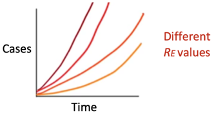
Figure 1: Cumulative number of cases over time for different Re values. Human behavior+virus behavior∝Re∝# cases over time

We can simplify our understanding of RE even further by breaking its relation down to “virus behaviors” and “human behaviors”.

𝐻𝑢𝑚𝑎𝑛 𝑏𝑒ℎ𝑎𝑣𝑖𝑜𝑟𝑠+𝑣𝑖𝑟𝑢𝑠 𝑏𝑒ℎ𝑎𝑣𝑖𝑜𝑟𝑠∝𝑅𝑒∝# 𝑐𝑎𝑠𝑒𝑠 𝑜𝑣𝑒𝑟 𝑡𝑖𝑚𝑒

Virus behavior is related to any virus property that is more or less constant and, usually, out of human control. This refers to the infectious period, incubation period, and infectivity, to name a few. The term infectivity encompasses the virus’ ability to inoculate, replicate within a host, its susceptibility within a host, and immune response. The terms incubation period and infectious period are discussed below.

Human behavior is related to cultural and social norms. These are more or less dynamic. The goal of public health is to influence human behavior to decrease the Re and ultimately slow the spread of a virus. This is why “flattening the curve” is so important. By staying at home and maintaining social distancing, the Re effectively decreases.

Rt(time-varying effective reproduction number)

The effective reproduction number can also be reported in a time-based fashion. There are numerous models described, however most of them use our knowledge of new and cumulative cases, the incubation period, as well as the serial interval distribution (described below). In some of the more sophisticated models, Rt is also adjusted for the effect of changes in testing practices. Most of these models are right-censored, meaning that today’s data is only informative of case data provided weeks leading up to it. For an example of predictive Rt modelling, see below (Figure 2). These models provide us a crude measure of where the pandemic is heading: If the Rt is close to 1 or less than 1, the number of new cases will begin to stabilize or decrease. This type of modelling helps inform public health officials when to ease control measures.

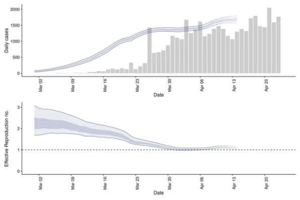
Figure 2: (Top) Confirmed Canadian cases and their estimated date of infection. (Bottom) Time-varying effective reproduction number with 90% confidence intervals (light ribbon). Source: https://epiforecasts.io/covid/posts/national/canada/

Incubation period

This is the period between exposure and appearance of the first symptoms. The incubation period can inform several important public health measures for monitoring, surveillance, control, and modeling. Thus, it is paramount that the incubation period estimate is an informed, evidence-based one. Usually, this involves screening infected populations on their symptom onset, possible initial exposure and case detection. Early in an epidemic, this can be challenging to estimate, especially with few cases. Transmission dynamics and epicurve modeling (Figure 3) can help identify a reasonable range. The incubation period of COVID-19 is estimated to be anywhere between 2 and 14 days, where only a few have presented with first symptoms less than 2 days and beyond 14 days. The upper end of the incubation period is often used by public health to determine the quarantine period for communicable diseases.

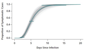
Figure 3: Transmission dynamics of the first 425 confirmed cases in Wuhan, China to determine the epidemiologic characteristics of COVID-19. Copied from NEJM 2020; 382:1199-1207.

Infectious period

In contrast, the infectious period refers to the period in which the person may infect others. More often than not, individuals become infectious during the incubation period when they may not manifest clinical signs or symptoms (Figure 4). A closely related term, viral shedding, has to do with the number of viral particles an individual sheds during the time they are infectious. Viral shedding for SARS-CoV-2 is thought to be highest early in the infectious period and may overlap the incubation period. Importantly, public health messaging has been clear: anyone with close contacts or suspected infection should self-isolate themselves for a period of time to ensure they don’t infect others.

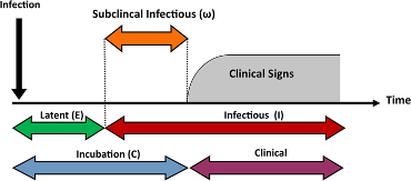
Figure 3: Distinct periods of infectious diseases. Copied from Sci Rep 9, 2707 (2019).

Serial interval

The serial interval is the time from onset of symptoms in one infected individual to the time of symptom onset in the case(s) they infect. When the serial interval is shorter than the incubation period, transmission is likely to occur in the incubation period. In the case of COVID19, the mean serial interval is shorter than the mean incubation period, suggesting that transmission can occur before individuals realize they are symptomatic.

Case fatality rate (CFR)

The case fatality rate (CFR) is simply the number of people who died of COVID19 divided by the total number of diagnosed cases.

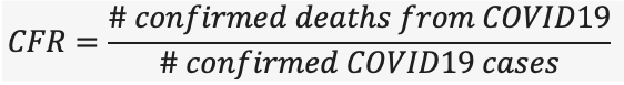
Based on the equation above, it is important to note that CFR is the ratio between confirmed deaths and confirmed cases, NOT total cases. The CFR is very easy to miscalculate; early in an epidemic, cases may be identified by those who have severe disease or those who die. Many individuals who may have the disease but have mild symptoms go undiagnosed, thus the CFR may be lower than what is reported. The CFR is also determined by the scale of testing efforts in a given population.

What we really want to know is that if someone is infected with COVID19, how likely is it that they will die. The answer to that is captured in part by the infection fatality rate (IFR).

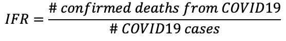
The total number of COVID19 cases is not known, and we may never know the true number of COVID19 cases. However, researchers can estimate the total number of cases through predictive models. It stands that the IFR is always lower than the CFR, and that the CFR will usually overestimate the true risk of death from the virus.

If we go back to the concept of CFR, a common misconception is that the CFR is a stable number, however, it often reflects the severity of the disease in one particular time, in a particular population, and in the right context. The CFR is usually the highest early on in an outbreak, then as testing ramps up and cases start to taper off, the CFR declines. The current CFR for COVID19 in Canada is 5.4% and globally 6.9% (as of April 26, 2020. As daily cases and deaths emerge, the CFR will be a moving target and may overestimate (if too many cases yet to be diagnosed) or underestimate (if most deaths are not captured early in the pandemic). For example, during the SARS-CoV outbreak in 2002, the CFR initially reported to be 5% during earlier stages, but had risen to 10% by the end of the pandemic.

CFR accuracy

While the CFR is challenging to accurately estimate in real-time, there are perhaps pockets of scenarios in the world that provide us an example of truer estimates.

Take Iceland for example; the country’s robust deCODE genetics program has allowed them to implement early and aggressive testing, to the point that they have screened more than 60,000 tests per million people, more than any country in the world. Their results have revealed a CFR thus far of approximately 0.5%. Interestingly, over 50% of positive cases were asymptomatic, confirming multiple studies that predicted asymptomatic carriers of COVID-19.

The Diamond Princess cruise ship is another example where a closed community can provide an estimate of the CFR. The cruise was supposed to finish a 14-day course on February 4^th, however, Japanese health officials ordered a quarantine when at least 10 passengers tested positive. By the end of it, nearly 3000 of the approximate 3700 passengers and crew members were tested. The CFR and IFR was estimated to be 2.3% and 1.2% respectively.

Interpreting these results at face value is fraught with problems. For example, these demographics are not the same across different nations and public health measures and testing capacity vary amongst different countries. With respect to the cruise ship, one can argue that those individuals likely are at a higher socioeconomic status and have limited comorbidities that can allow them to travel for more than 2 weeks. So while these CFR numbers provide interesting estimates of overall fatalities within a closed community, they cannot be generalizable.

Modeling pandemics, are we in the right direction?

With all of this information, how does one tell if this pandemic is heading in the right direction? Fortunately, we have various predictive transmission models that can estimate the spread of the variations amongst a population over time. One model that is commonly used in epidemiology is the SIR model, or susceptible-infected-recovered, that projects the theoretical number of infected people with an infectious disease in a closed population (such as the hospital) over time. Many complicated and modified versions of the SIR model have been proposed to more accurately reflect the biology of a given disease.

The Kermack-McKendrick model is a more simple form of the SIR model. It uses a triply-coupled non-linear differential equation.

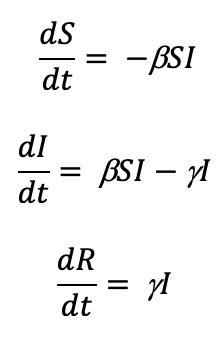
where S is the number of susceptible people (in the beginning of a pandemic this is essentially everyone), I is the number of people infected, R is the number of people who have recovered and developed immunity. b is the infection rate and closely related to the R0, and g is the recovery rate. We are primarily concerned about the number of people infected, so let’s focus on the second equation. If we assume early in a novel virus pandemic that there are very few recovered and immunized, those that get infected can be estimated by:

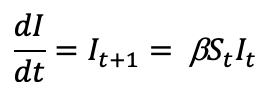
Where t can be an arbitrary amount of time (days, hours, weeks, etc.). As mentioned above, b is the infection rate and is closely related to the R_e and control measures such as “physical distancing”. This means that b is highly impacted by social interventions such as physical distancing as it is one of the most effective public health interventions in slowing the spread of SARS-CoV-2. In fact, many models are predicted based on the amount of “physical distancing” that takes place. For example, a b of 0.5 means that 50% of susceptible people (R_t) that are in contact with an infected person (I_t ) will become infected.

Model projections generally appear as below (Figure 5), where the more effective the social intervention (such as physical distancing and enhanced case detection), the fewer cases over time and slower the rate of new cases over time. In the example below, green would represent the most effective social intervention:

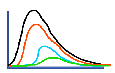
Figure 5: Projected hospital census for various physical distancing effectiveness

For examples of various online COVID-19 projection models, see below:

1. 613covid.ca: daily projected hospital census for Ottawa (https://613covid.ca)

2. COVID-19-MC: Predicting healthcare resource needs in Ontario (https://www.covid-19-mc.ca/interactive-model)

3. CHIME: COVID-19 Hospital Impact Model for Epidemics (https://penn-chime.phl.io/)

Additional ways to identify strain on our healthcare system caused by the virus is by looking at daily admissions and capacity metrics. These include, but not limited to: admission rates, ICU admission rates including ventilated and non-ventilated patients, remaining bed and ventilator capacity, as well as case-specific mortality. A commonly reported number is the doubling time, the time it takes to double the cases of COVID-19 in the hospital. This is a dynamic number that is dependent on the influx of positive cases that get admitted. The doubling time usually decreases when fewer susceptible cases are present and preventive measures are in place.

In contrast, the commonly reported cumulative positive cases or new cases per day often misleads the public because these numbers are dependent on factors such as our testing capacity, testing turnaround time, and how broad our screening criteria is. The metrics and predictive modeling described above provide a more accurate picture on which direction the pandemic is heading. These models not only assist hospital stakeholders with respect to surge capacity planning, but also aids public health officials to make important and often difficult decisions when it comes to easing control measures such as physical distancing and re-opening the economy

References

Lauer SA, Grantz KH, Bi Q, et al. The Incubation Period of Coronavirus Disease 2019 (COVID-19) From Publicly Reported Confirmed Cases: Estimation and Application. Ann Intern Med. 2020
Li Q, Guan X, Wu P, Wang X, Zhou L, Tong Y, et al. Early transmission dynamics in Wuhan, China, of novel coronavirus-infected pneumonia. N Engl J Med. 2020 Jan 29
Linton NM, Kobayashi T, Yang Y, Hayashi K, Akhmetzhanov AR, Jung S-M, Yuan B, Kinoshita R, Nishiura H. Epidemiological characteristics of novel coronavirus infection: a statistical analysis of publicly available case data. medRxiv. 2020 Jan 26.
Arzt, J., Branan, M.A., Delgado, A.H. et al. Quantitative impacts of incubation phase transmission of foot-and-mouth disease virus. Sci Rep 9, 2707 (2019)
He, X., Lau, E.H.Y., Wu, P. et al. Temporal dynamics in viral shedding and transmissibility of COVID-19. Nat Med (2020).
Nishiura H, Linton NM, Akhmetzhanov AR. Serial interval of novel coronavirus (COVID-19) infections. Int J Infect Dis. 2020 Mar 4
Du Z, Wang L, Chauchemez S, Xu X, Wang X, Cowling BJ, et al. Risk for transportation of 2019 novel coronavirus disease from Wuhan to other cities in China. Emerg Infect Dis. 2020;26(5)
Gudbjartsson DF, Helgason A, Jonsson H, et al. Spread of SARS-CoV-2 in the Icelandic Population. NEJM (2020).
Russel TW, Hellewell J, Jarvis CI, van zandvoort K, Abbott S, Ratnayake R, CMMID COVID-19 working group, Flasche S, Eggo RM, Edmunds WJ, Kucharski AJ. Estimating the infection and case fatality ratio for coronavirus disease (COVID-19) using age-adjusted data from the outbreak on the Diamond Princess cruise ship, February 2020. Euro Surveill. 2020; 25(12):pii=2000256.
Jones, D. S. and Sleeman, B. D. Ch. 14 in Differential Equations and Mathematical Biology. London: Allen & Unwin, 1983
Tuite A, Fisman DN, Greer AL. Mathematic modeling of COVID-19 transmission and mitigation strategies in the population of Ontario, Canada. March 2020.
https://www.medrxiv.org/content/10.1101/2020.03.24.20042705v1